The Uses And Limits Of Volatility
|
Posted: Jun 6, 2010 |
|
|
Filed under
Financial Theory
Investing Basics
Investment
Stock Analysis
Stocks
Volatility
|

David Harper
Volatility = Annualized Standard Deviation
Unlike implied volatility - which belongs to option pricing theory and is a forward-looking estimate based on a market consensus - regular volatility looks backward. Specifically, it is the annualized standard deviation of historical returns.
Traditional risk frameworks that rely on standard deviation generally assume that returns conform to a normal bell-shaped distribution. Normal distributions give us handy guidelines: about two-thirds of the time (68.3%), returns should fall within one standard deviation (+/-); and 95% of the time, returns should fall within two standard deviations. Two qualities of a normal distribution graph are skinny "tails" and perfect symmetry. Skinny tails imply a very low occurrence (about 0.3% of the time) of returns that are more than three standard deviations away from the average. Symmetry implies that the frequency and magnitude of upside gains is a mirror image of downside losses. (For more on volatility, check out Volatility's Impact On Market Returns.)</INVESTOPEDIACONTENT>
Consequently, traditional models treat all uncertainty as risk, regardless of direction. As many people have shown, that's a problem if returns are not symmetrical - investors worry about their losses "to the left" of the average, but they do not worry about gains to the right of the average.
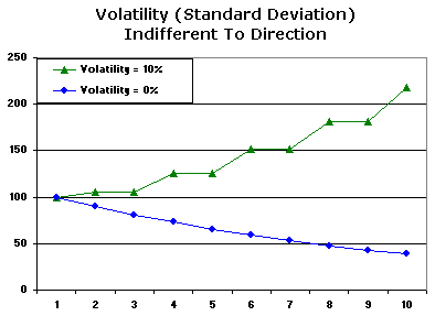
We illustrate this quirk below with two fictional stocks. The falling stock (blue line) is utterly without dispersion and therefore produces a volatility of zero, but the rising stock - because it exhibits several upside shocks but not a single drop - produces a volatility (standard deviation) of 10%.
 |
Theoretical Properties
When we calculate the volatility for the S&P 500 index as of January 31, 2004, we get anywhere from 14.7% to 21.1%. Why such a range? Because we must choose both an interval and a historical period. In regard to interval, we could collect a series of monthly, weekly or daily (even intra-daily) returns. And our series of returns can extend back over a historical period of any length, such as three years, five years or 10 years. Below, we've computed the standard deviation of returns for the S&P 500 over a 10-year period, using three different intervals:
 |
Notice that volatility increases as the interval increases, but not nearly in proportion: the weekly is not nearly five times the daily amount and monthly is not nearly four times the weekly. We've arrived at a key aspect of random walk theory: standard deviation scales (increases) in proportion to the square root of time. Therefore, if the daily standard deviation is 1.1%, and if there are 250 trading days in a year, the annualized standard deviation is the daily standard deviation of 1.1% multiplied by the square root of 250 (1.1% x 15.8 = 18.1%). Knowing this, we can annualize the interval standard deviations for the S&P 500 by multiplying by the square root of the number of intervals in a year:
 |
Another theoretical property of volatility may or may not surprise you: it erodes returns. This is due to the key assumption of the random walk idea: that returns are expressed in percentages. Imagine you start with $100 and then gain 10% to get $110. Then you lose 10%, which nets you $99 ($110 x 90% = $99). Then you gain 10% again, to net $108.90 ($99 x 110% = $108.9). Finally, you lose 10% to net $98.01. It may be counter-intuitive, but your principal is slowly eroding even though your average gain is 0%!
If, for example, you expect an average annual gain of 10% per year (i.e. arithmetic average), it turns out that your long-run expected gain is something less than 10% per year. In fact, it will be reduced by about half the variance (where variance is the standard deviation squared). In the pure hypothetical below, we start with $100 and then imagine five years of volatility to end with $157:
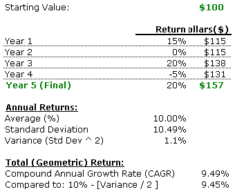 |
The average annual returns over the five years was 10% (15% + 0% + 20% - 5% + 20% = 50% ÷ 5 = 10%), but the compound annual growth rate (CAGR, or geometric return) is a more accurate measure of the realized gain, and it was only 9.49%. Volatility eroded the result, and the difference is about half the variance of 1.1%. These results aren't from a historical example, but in terms of expectations, given a standard deviation of ![]() (variance is the square of standard deviation,
(variance is the square of standard deviation, ![]() ^2) and an expected average gain of
^2) and an expected average gain of ![]() , the expected annualized return is approximately
, the expected annualized return is approximately ![]() - (
- (![]() ^2 ÷ 2).
^2 ÷ 2).
Are Returns Well Behaved?
The theoretical framework is no doubt elegant, but it depends on well-behaved returns. Namely, a normal distribution and a random walk (i.e. independence from one period to the next). How does this compare to reality? We collected daily returns over the last 10 years for the S&P 500 and Nasdaq below (about 2,500 daily observations):
 |
 |
As you may expect, the volatility of Nasdaq (annualized standard deviation of 28.8%) is greater than the volatility of the S&P 500 (annualized standard deviation at 18.1%). We can observe two differences between the normal distribution and actual returns. First, the actual returns have taller peaks - meaning a greater preponderance of returns near the average. Second, actual returns have fatter tails. (Our findings align somewhat with more extensive academic studies, which also tend to find tall peaks and fat tails; the technical term for this is kurtosis). Let's say we consider minus three standard deviations to be a big loss: the S&P 500 experienced a daily loss of minus three standard deviations about -3.4% of the time. The normal curve predicts such a loss would occur about three times in 10 years, but it actually happened 14 times!
These are distributions of separate interval returns, but what does theory say about returns over time? As a test, let's take a look at the actual daily distributions of the S&P 500 above. In this case, the average annual return (over the last 10 years) was about 10.6% and, as discussed, the annualized volatility was 18.1%. Here we perform a hypothetical trial by starting with $100 and holding it over 10 years, but we expose the investment each year to a random outcome that averaged 10.6% with a standard deviation of 18.1%. This trial was done 500 times, making it a so-called Monte Carlo simulation. The final price outcomes of 500 trials are shown below:
 |
A normal distribution is shown as backdrop solely to highlight the very non-normal price outcomes. Technically, the final price outcomes are lognormal (meaning that if the x-axis were converted to natural log of x, the distribution would look more normal). The point is that several price outcomes are way over to the right: out of 500 trials, six outcomes produced a $700 end-of-period result! These precious few outcomes managed to earn over 20% on average, each year, over 10 years. On the left hand side, because a declining balance reduces the cumulative effects of percentage losses, we only got a handful of final outcomes that were less than $50. To summarize a difficult idea, we can say that interval returns - expressed in percentage terms - are normally distributed, but final price outcomes are log-normally distributed. (Learn more about this type of analysis in Multivariate Models: The Monte Carlo Analysis.)
Finally, another finding of our trials is consistent with the "erosion effects" of volatility: if your investment earned exactly the average each year, you would hold about $273 at the end (10.6% compounded over 10 years). But in this experiment, our overall expected gain was closer to $250. In other words, the average (arithmetic) annual gain was 10.6%, but the cumulative (geometric) gain was less.
It is critical to keep in mind that our simulation assumes a random walk: it assumes that returns from one period to the next are totally independent. We have not proved that by any means, and it is not a trivial assumption. If you believe returns follow trends, you are technically saying they show positive serial correlation. If you think they revert to the mean, then technically you are saying they show negative serial correlation. Neither stance is consistent with independence.
Conclusion
Volatility is annualized standard deviation of returns. In the traditional theoretical framework, it not only measures risk, but affects the expectation of long-term (multi-period) returns. As such, it asks us to accept the dubious assumptions that interval returns are normally distributed and independent. If these assumptions are true, high volatility is a double-edged sword: it erodes your expected long-term return (it reduces the arithmetic average to the geometric average), but it also provides you with more chances to make a few big gains. (For further reading, check outImplied Volatility: Buy Low And Sell High.)
He is the principal of Investor Alternatives, a firm that conducts quantitative research, consulting (derivatives valuation), litigation support and financial education.
Read more: http://www.investopedia.com/articles/04/021804.asp#ixzz1OyWeL0vJ